Knowledge Graphs

Following recent developments in natural language processing and machine learning, knowledge graphs have emerged as a powerful data modeling tool, capable of breaking down abstract concepts into networks of simpler, interrelated concepts. They are a type of graph data structure in which nodes represent simple concepts identified within audio files, i.e. "lion" and "wind," and edges represent relationships between them. Knowledge graphs extend this concept further by using edges to convey the knowledge of large-scale real world data, connecting shared characteristics called “features” between data points. For unstructured data, the raw input is run through a data process- ing pipeline that extracts relationships, producing interpretable entities (nodes) and connections (edges) used to construct the graph.

Applications to Bioacoustics

Using an unsupervised data processing pipeline to create knowledge graphs, we can discover and connect features within large batches of unstructured bioa- coustic audio data sets. Our Python-based data processing pipeline consists of four major steps. First, the pipeline begins by loading the audio files and all corresponding annotations. The audio is then passed through standard preprocessing and denoising steps using a Deep Convolutional Neural Network architecture. After preprocessing, each file is divided into five-second segments, or "chunks," which remain linked to the annotations of the original recording. Third, the segmented audio clips are processed by an autoencoder. Autoencoders are unsupervised machine learning models that compress data into a simplified latent representation and, if needed, reconstruct the original input from that compressed form. Each time the pipeline receives an au- dio chunk, the autoencoder trains by repeatedly compressing and decompressing the input. Our method relies solely on the compressed representations after the model has completed training. Once a denoised chunk has been encoded into a vector embedding containing only the most essential distinguishing character- istics—such as "dog" or "rainy season"—these embeddings are clustered so that chunks with similar features are grouped together. Finally, a graph is generated from the encoded data and visualized using the external visualization library D3. At this stage, the annotations primarily serve to support the visualization.

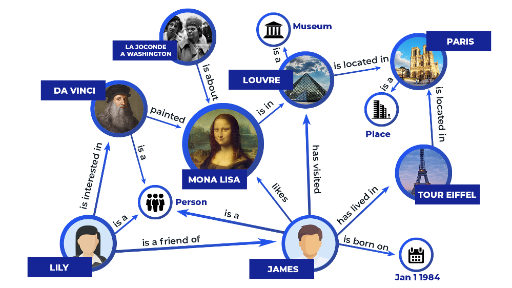
As shown above, the knowledge graph is composed of two types of nodes: those representing the five second audio chunks and those representing features such as time of day, season, species, or weather characteristics. A feature node is connected to one or more audio-chunk nodes by an edge whenever those chunks exhibit that feature. Through these connections, the graph captures both the characteristics present in each audio segment and the relationships among segments that share similar attributes. A feature node is linked to multiple audio chunks - for example, a node labeled “lion” reveals similarities or previously overlooked patterns across recordings. Visualizing these relationships in a graph provides an intuitive way to uncover new connections that may not be immediately apparent from the raw audio alone. In particular, representing relationships within under-labeled soundscape data enables ecologists to gain deeper insight into the environments they study and to develop new hypotheses through exploration of the generated feature-audio knowledge graph.